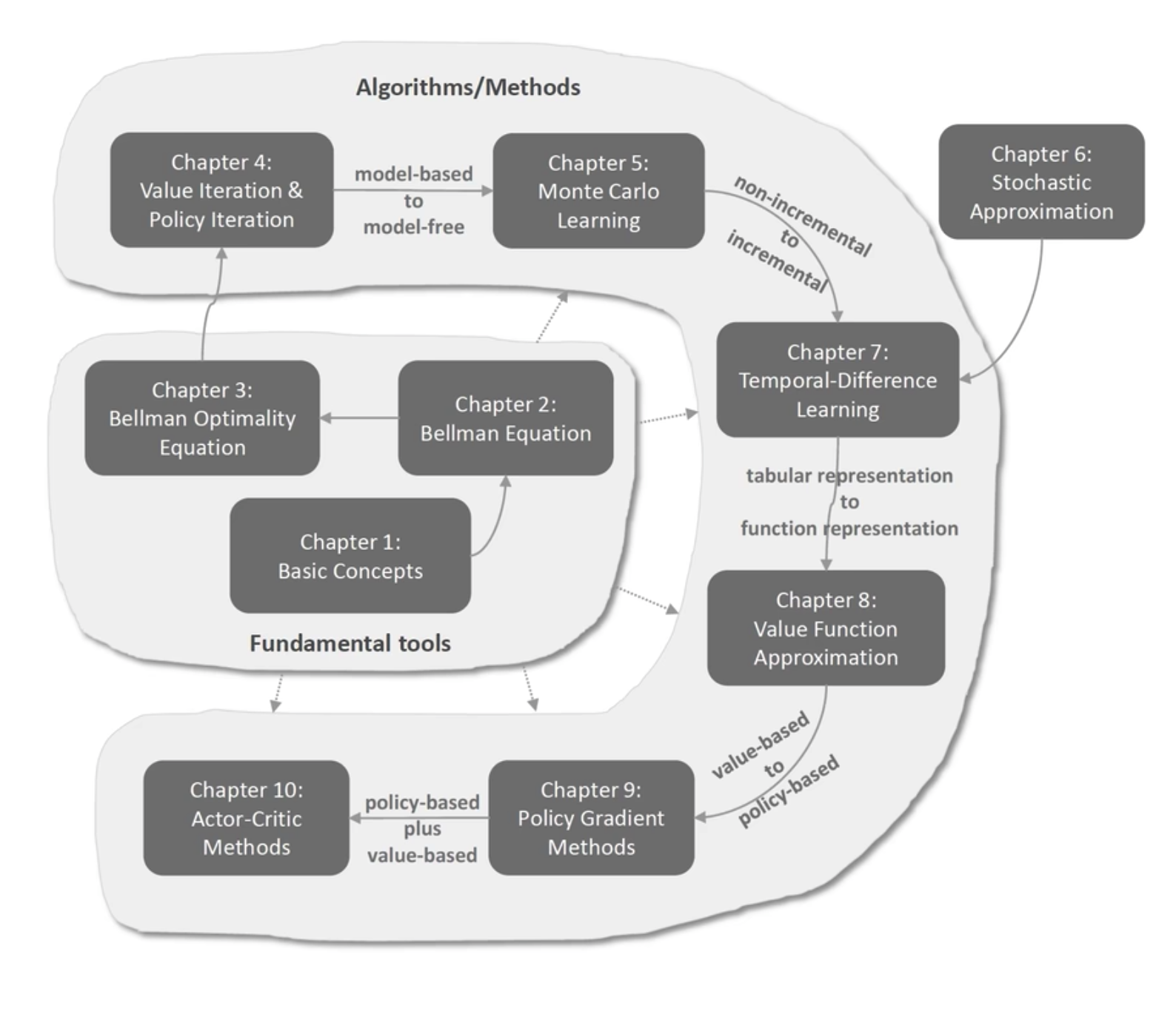
西湖大学赵世钰老师《强化学习的数学原理》笔记整理:基本概念(P4-P5)。
1. Fundamental concepts in RL
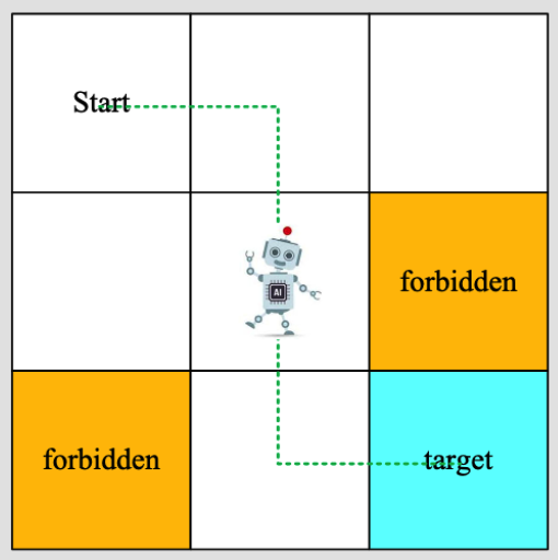
本课程采用grid-world示例,特点如下:
- 网格有不同的类型(可进入cell、禁止区域cell、目标cell)
- 有边界
- 机器人可以在水平/竖直方向移动,不可以斜着走
- 给定一个起始点,机器人需要寻找一个“最优”的到达目标的路线
1.1 State
state是agent相对于环境(environment)的状态(status)。在grid-world中,state是agent所处的位置(共有9个state:$s_1,s_2,...,s_9$)
状态空间 State space: $\mathcal{S} = \{s_i\}_{i=1}^9$
1.2 Action
对每一个state,action表示agent可以采取的行为,(共有5个action:$a_1,a_2,a_3,a_4,a_5$,分别表示向上、右、下、左、保持不动)。
动作空间和状态state有关,因此可以描述为:$\mathcal{A}(s_i) = \{a_i\}_{i=1}^5$
1.3 State transition
Agent采取了一个action,由一个state转移到另一个state的过程,称为state transition,如:
$$ s_1 \overset{a_2}{\rightarrow} s_2 $$
再比如,在$s_1$采取$a_1$的情况下,agent仍然停留在$s_1$,因为触到了边界。
$$ s_1 \overset{a_1}{\rightarrow} s_1 $$
对于forbidden area,假设agent位于$s_5$,采取$a_2$,下一个状态可能的情况:
- case 1:forbidden area $s_6$可以进入,但有惩罚:$s_5 \overset{a_2}{\rightarrow} s_6$
- case 2:forbidden area $s_6$不可以进入,agent仍然停留在$s_5$:$s_5 \overset{a_2}{\rightarrow} s_5$
本课程中,我们采取case 1的设定(更一般化,更难些)。
State transition可以用表格形式展示出来:
| $a_1$ | $a_2$ | $a_3$ | $a_4$ | $a_5$ | |
|---|---|---|---|---|---|
| $s_1$ | $s_1$ | $s_2$ | $s_4$ | $s_1$ | $s_1$ |
| $s_2$ | $s_2$ | $s_3$ | $s_5$ | $s_1$ | $s_2$ |
| $s_3$ | $s_3$ | $s_3$ | $s_6$ | $s_2$ | $s_3$ |
| $s_4$ | $s_1$ | $s_5$ | $s_7$ | $s_4$ | $s_4$ |
| $s_5$ | $s_2$ | $s_6$ | $s_8$ | $s_4$ | $s_5$ |
| $s_6$ | $s_3$ | $s_6$ | $s_9$ | $s_5$ | $s_6$ |
| $s_7$ | $s_4$ | $s_8$ | $s_7$ | $s_7$ | $s_7$ |
| $s_8$ | $s_5$ | $s_9$ | $s_8$ | $s_7$ | $s_8$ |
| $s_9$ | $s_6$ | $s_9$ | $s_9$ | $s_8$ | $s_9$ |
但表格只能表示确定性的场景(使用受限)。因此,更一般的地,使用state transition probability来表示:
即:在状态$s_i$采取动作$a_j$的情况下,下一个状态为$s_k$的概率为:
$$p(s_k \mid s_i,a_j) = p$$
其中$p$为概率值。
比如:
$$ p(s_2 \mid s_1, a_1)=1 $$
$$ p(s_i \mid s_1,a_2) = 0 \quad \forall i \neq 2 $$
1.4 Policy
在某一个state上,告诉agent应该采取什么action。直观地,使用箭头表示策略:

1.4.1 数学表达
针对状态$s_1$,采取动作$a_1 ... a_5$的概率为:
$$ \pi(a_1 \mid s_1) = 0 $$
$$ \pi(a_2 \mid s_1) = 1 $$
$$ \pi(a_3 \mid s_1) = 0 $$
$$ \pi(a_4 \mid s_1) = 0 $$
$$ \pi(a_5 \mid s_1) = 0 $$
这种称为确定性策略。当然,也可以是随机策略,比如:
$$ \pi(a_1 \mid s_1) = 0 $$
$$ \pi(a_2 \mid s_1) = 0.5 $$
$$ \pi(a_3 \mid s_1) = 0.5 $$
$$ \pi(a_4 \mid s_1) = 0 $$
$$ \pi(a_5 \mid s_1) = 0 $$
每一个action都有其概率,我们可以将概率为0的省略:
$$ \pi(a_2 \mid s_1) = 0.5 $$
$$ \pi(a_3 \mid s_1) = 0.5 $$
1.4.2 Policy的表格化描述:
| $a_1(up)$ | $a_2(right)$ | $a_3(down)$ | $a_4(left)$ | $a_5(stay)$ | |
|---|---|---|---|---|---|
| $s_1$ | 0 | 0.5 | 0.3 | 0 | 0 |
| $s_2$ | 0 | 0 | 1 | 0 | 0 |
| $s_3$ | 0 | 0 | 0 | 1 | 0 |
| $s_4$ | 0 | 1 | 0 | 0 | 0 |
| $s_5$ | 0 | 0 | 1 | 0 | 0 |
| $s_6$ | 0 | 0 | 1 | 0 | 0 |
| $s_7$ | 0 | 1 | 0 | 0 | 0 |
| $s_8$ | 0 | 1 | 0 | 0 | 0 |
| $s_9$ | 0 | 0 | 0 | 0 | 1 |
1.5 Reward
Reward是agent在采取一个action后,得到的一个标量(real number):
- reward为正,表示采取上述action得到了奖励
- reward为负,表示采取上述action得到了惩罚
当然,reward也可以为0,表示没有惩罚;正reward也可以作为惩罚(只是作为一种数学上的标记)。
在grid-world中,我们设定reward为:
- agent穿越了边界,$r_{bound} = -1$
- agent进入了forbidden cell,$r_{forbid} = -1$
- agent进入了target cell,$r_{target} = 1$
- 否则,$r = 0$
reward可以理解成人机接口(human-machine interface),我们可以通过设计reward来引导agent的行为,实现我们想要的目标。
1.5.1 reward的表格化描述:
| $a_1(up)$ | $a_2(right)$ | $a_3(down)$ | $a_4(left)$ | $a_5(stay)$ | |
|---|---|---|---|---|---|
| $s_1$ | $r_{bound}$ | 0 | 0 | $r_{bound}$ | 0 |
| $s_2$ | $r_{bound}$ | 0 | 0 | 0 | 0 |
| $s_3$ | $r_{bound}$ | $r_{bound}$ | $r_{forbid}$ | 0 | 0 |
| $s_4$ | 0 | 0 | $r_{forbid}$ | $r_{bound}$ | 0 |
| $s_5$ | 0 | $r_{forbid}$ | 0 | 0 | |
| $s_6$ | 0 | $r_{bound}$ | $r_{target}$ | 0 | $r_{forbid}$ |
| $s_7$ | 0 | 0 | $r_{bound}$ | $r_{bound}$ | $r_{forbid}$ |
| $s_8$ | 0 | $r_{target}$ | $r_{bound}$ | $r_{forbid}$ | 0 |
| $s_9$ | $r_{forbid}$ | $r_{bound}$ | $r_{bound}$ | 0 | $r_{target}$ |
1.5.2 数学表达:
$$ p(r=1 \mid s_1,a_1)=1 $$
$$ p(r \neq -1 \mid s_1,a_1) = 0 $$
reward也可能是具有随机性的。reward依赖于当前的状态和action,而不是下一个状态,例子:$(s_1,a_1)$和$(s_1,a_5)$得到的reward不应该相同。
1.6 Trajectory
Trajectory是agent在环境中的一条轨迹,是一个序列(state-action-reward链):
$$s_1 \underset{r=0}{\stackrel{a_2}{\longrightarrow}} s_2 \underset{r=0}{\stackrel{a_3}{\longrightarrow}} s_5 \underset{r=0}{\stackrel{a_3}{\longrightarrow}} s_8 \underset{r=1}{\stackrel{a_2}{\longrightarrow}} s_9$$
这个trajectory的return是链上所有action得到的reward的加和。
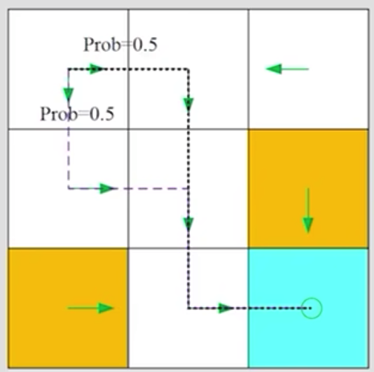
对比两个trajectory:

哪个policy比较好?
- 直觉上,左侧的更好,因为它避开了forbidden cell
- 数学上,左侧的更好,因为它的return更大
- return可以用于评估policy的好坏
trajectory也可能是无限长的,比如:
$$s_1 \overset{a_2}{\rightarrow} s_2 \overset{a_3}{\rightarrow} s_5 \overset{a_3}{\rightarrow} s_8 \overset{a_2}{\rightarrow} s_9 \overset{a_5}{\rightarrow} s_9 \overset{a_5}{\rightarrow} s_9 ...$$
这个trajectory的return是$0+0+0+1+1+1+...=\infty$,这个return是无限大的,是发散的。如何解决这个问题?
可以通过引入discount rate $\gamma$来解决,$\gamma \in [0,1]$:
$$ \mathrm{discount\quad return} = 0 + \gamma 0 + \gamma^2 0 + \gamma^3 1 + \gamma^4 1 + \gamma^5 1 + ... = \gamma^3 \frac{1}{1-\gamma}$$
此时:
- return收敛
- $\gamma$可用于平衡长程和短程reward
- $\gamma$越大,越重视未来的reward(短视)
- $\gamma$越小,越重视当前的reward(远视)
1.7 Episode
Agent根据一个policy与环境交互时,agent可能会停在一个最终状态(terminal state)上,对应的trajectory(一般假定是有限的)称为一个episode(或称一个trial)。对应的任务称为episodic task。
有一些任务可能没有terminal state,此时agent会永远和环境交互下去,这种task称为continuing task。
在grid-world中,在到达target后,我们应该停下来吗?
本课程不区分对待episodic和continuing tasks的方法,(实际是将episodic task转换成continuing task)。两种方法:
-
把target state认为是一个特殊的absorbing state
在设置其stage transition probability时,如果当前状态就是target的状态,那么不论采取什么样的action它都会再回到这个状态。或者说在这个状态的时候,就没有其它的action。 我可以修改它的action space,让它的action只有留在原地这样一个action,之后所得到的所有的reward全都是0;
-
认为target state是一个普通的状态
策略足够好的话,agent会一直停留在这个state,(收集正的reward),策略不好的话,它可能跳出这个state;
本课程采用第二种处理方式,它无需对target进行区别对待,也更一般化。
2. Formalize the concepts in the context of MDP
Key elements of MDP:
- 包含很多sets
- state: the set of states $\mathcal{S}$
- Action: the set of actions $\mathcal{A(s)}$ associated with state $s \in \mathcal{S}$
- Reward: the set of rewards $\mathcal{R(s,a)}$
- probability distribution
- State transition probability: 由状态$s$经过action$a$跳到状态$s'$的概率$p(s'\mid s,a)$
- Reward probability: 在状态$s$采取action $a$得到reward $r$的概率$p(r\mid s,a)$
- policy: 在状态$s$采取action $a$的概率$\pi(a\mid s)$
- Markov property: memoryless property
- $p(s_{t+1}\mid a_{t+1},s_t,...,a_1,s_0)=p(s_{t+1}\mid a_{t+1},s_t)$
- $p(r_{t+1}\mid a_{t+1},s_t,...,a_1,s_0)=p(r_{t+1}\mid a_{t+1},s_t)$
什么是MDP:
- M: Markov property
- D: policy
- P: sets & probability distribution
回到grid-world例子,可以抽象为一个更一般的模型:markov process(当policy确定时,MDP就变成了markov process)。
本节课结束,下节课会介绍贝尔曼公式。